When Did the Waters Part?

A Quantitative Reconstruction of the Post-Catastrophe Climate, Sea Level, and Dispersal Infrastructure Part Two of the Diaspora Series The paper builds on the qualitative framework established in "Where Did the Dove Find Peace?" (Part One) and should be read as a continuation of that work.

← Return to the Diaspora Series

The Clock Starts

The first paper in this series established ten propositions describing the post-catastrophe recovery as a practical engineering problem. The tectonic “main event” was brief and violent. The landscape resumed rather than restarted. The new warm ocean basins were an inevitable consequence. The ice age followed necessarily. Those propositions were qualitative — practical inferences from the Genesis account treated as an engineering specification. This paper examines whether the specifications are plausible by making them quantitative. Almost every number in this paper derives from a single source: the velocity of the tectonic plates as a function of time. The one exception is the magnitude of the thermal contraction, which comes from the heat budget of the foundational standalone rather than from the velocity curve — though velocity still sets when that heat is released, and so when the contraction happens. That velocity curve — inherited from the foundational standalone and constrained by the observed continental displacement of approximately 5,000 km — determines the rate of ocean heating, the depth of new basins, the height of rising mountains, the intensity of volcanic forcing, and the area of new seafloor. Five outputs from one equation — plate velocity as a function of time — constrained by the observed continental separation and the peak velocity the force balance produces. The question is not whether the waters parted. The first paper established that they did — mountains rose, basins deepened, ice accumulated. The question is when. When did the sea level drop far enough to connect Asia to North America? When did the corridor to Australia open? When did the bridges close, locking each continent's founding roster in place? The answer, as it turns out, is early — but not instantaneous. The new ocean basins must first form solid lithosphere before they can deepen, and that sets the starting gun for the sea level drop. A critical point must be established before the numbers begin. The recovery does not start when the animals exit the ark at day 371. It does not start when the ark grounds at day 150. It starts during the catastrophe itself. Mountains thrust upward by plate convergence push above the water surface within weeks. Rain falls on exposed rock immediately. Salt washes from soil within days under extreme precipitation. Pioneer vegetation — from surviving root systems, not distant seed sources — resumes growth on volcanic ash within weeks of exposure. Under secondary succession accelerated by extreme precipitation and volcanic ash fertilization, pioneer vegetation on newly exposed highlands reaches measurable biomass within three to nine months. This is consistent with Krakatoa and Mount St. Helens recovery rates, and likely faster given surviving root systems rather than wind-dispersed seed colonization. By the time the ark grounds at day 150, the Tibetan Plateau has been catching rain and growing things for months. The Ethiopian Highlands, the Andes, and every other landmass above 3,000 meters are well into recovery. The olive leaf that the dove returns at day 272 is not the beginning of recovery. It is a measurement taken months into a recovery already well underway. By the time the ark's passengers descend the ramp at day 371, the highest terrain has supported active plant growth for the better part of a year. The world they walk into is not post-catastrophe. It is mid-recovery.

The Velocity Profile

One Curve, Inherited

This paper does not build a velocity model. It uses the one developed in the foundational standalone, "What Broke the Foundations?", and takes nothing from the narrative that the physics does not already supply. What is inherited is a single exponential decay: v(t) = 12 km/yr × exp(−t / 417.5 yr). The peak comes from a force balance — cork-popping geometry, grain-size evolution, hydration and partial melt, each quantified from published experimental data. The decay constant is not chosen: the observed 5,000 km of continental separation, divided by that peak, fixes it at 417.5 years. No elapsed time enters the calculation, and no figure from the narrative enters it. What the specification contributes is shape, not parameters. The account records a violent onset followed by decline — severe at the start and subsiding thereafter, rather than steady or building toward a peak. That is the shape a decaying velocity profile has, and it is what the mechanism independently produces as the driving stress relaxes and the weakened pathways heal. It is a match in character, and this paper claims nothing more from it. The day-40 marker is about the water. The narrative's vocabulary shifts at day 40 from mabbul, the violent deluge, to mayim, waters. That is not a boundary in the plate velocity: on the inherited profile, velocity at day 40 has fallen by three hundredths of one percent, and by the end of the first year by two tenths. Nothing tectonic happens on that timescale. What does change on that timescale is the water, and the mechanism says why. Tsunamis are generated by impulsive displacement — meters of seafloor in seconds. Sustained plate motion at peak is 33 meters a day, and horizontal rather than vertical: not impulsive, and orders of magnitude too slow to raise a wave. It produces currents. The violent water is therefore front-loaded — the initial failure and the cascade around the basin perimeter — and a steadily declining separation velocity does not resupply it. What remains is not quiet. Basins of that size, once disturbed, oscillate: a Pacific-scale basin has a fundamental period of order forty hours, and water standing over a flooded continental interior far longer. That is a slow rocking rather than a train of waves, and discrete events at the subduction margins continue alongside it. But the regime after the first weeks is sloshing and current rather than repeated inundation — which is what the shift in the record describes, and it arrives while the plates are still moving at nearly full speed. The derivation and what is taken from it are set out in Appendix A.

The Warm Ocean

The catastrophe delivers an enormous quantity of heat to the ocean. The total energy delivered — fixed by the measured heat flux through the new basins, the solidus that marks the base of the solidified column, and the new-basin area — is approximately 1.80 × 10²⁸ joules. No volume calculation and no mass balance enters that budget: material below the solidification front is still there and still warm, and none of its heat reached the ocean. The full derivation, including the three-phase delivery mechanism (charging, boiling discharge, conductive tail) and the basin-resolved heat budget, is presented in Appendix F of the foundational standalone ("What Broke the Foundations?"). The thermal architecture is asymmetric. The Atlantic and Indian rift basins receive direct emplacement of new mantle material at the surface; their basin floors boil seawater at the 100°C surface boundary throughout the active discharge phase (approximately 310–478 years, depending on the effective boiling flux). The Pacific receives little direct tectonic heat — it is the remnant of the pre-event ocean, redistributing heat primarily through atmospheric and oceanic circulation. The Atlantic and Indian basins are lethally hot during Phase 1–2. The remnant ocean is not a contact surface — no new crust forms there and no mantle is exposed at its floor — so it receives no emplacement heat and warms only by transport. No temperature is quoted for it here: neither the exchange at the contacts nor the atmospheric return is quantified in that work, and a figure produced without them would be an assertion rather than a result. The biological consequences of this asymmetry — including marine biosphere survival in the Pacific, and the differential timing of recovery in the other basins — are developed in the paper “What Broke the Foundations?”. This paper does not simulate the three-basin SST distribution directly. The downstream analysis — sea level budget, bridge timing, corridor climates — depends on quantities (total ocean heat content, global atmospheric forcing, latitude-band temperature) that do not require basin-resolved ocean temperatures. The reader is again referred to the paper “What Broke the Foundations?”, Appendix F, for the full heat budget and basin-resolved treatment. What this paper does model directly is the atmospheric temperature response. The catastrophic event produces two forcings on the global atmosphere — volcanic aerosol cooling from sustained ridge eruption, and increased planetary albedo from extensive cloud cover over the boiling rift basins — that together drive a calibrated energy-balance-model response. That response is presented in the next section.

The Climate Forcing

The catastrophe imposes two large radiative forcings on the global atmosphere. The first is volcanic aerosol cooling. The second is increased planetary albedo from sustained cloud cover over the boiling rift basins. Both are tied to the velocity profile — both peak with the active discharge phase and decay as the system relaxes toward modern conditions. Volcanic forcing. During the active phase, the mid-ocean ridge system erupts continuously to produce new crust. The eruption rate is not a free parameter — it follows from the plate velocity. A fraction of this eruption is subaerial: continental arc volcanism at the Ring of Fire, plus flood basalt provinces along the separating margins. The subaerial fraction is the component that loads the atmosphere with sulfate aerosols. The basin emplacement is not radiatively inert, however: magma driven up under pressure and quenching against the boiling basin surface is a genuine sulfur source. That sulfur is largely scrubbed into the brine or rained out of the saturated lower atmosphere within a day rather than reaching the stratosphere, so its role is indirect — it feeds the cloud deck and is treated with the cloud-albedo term below, not with the subaerial forcing here. The effective volcanic forcing used here is approximately 60% of the original full-eruption-rate reference value of -10 W/m². This reduction reflects the subaerial fraction of total eruption (estimated at approximately 25–40% of total volume, scaled by the more explosive nature of catastrophic continental rifting), together with the rapid tropospheric washout that limits the residence time of tropospheric aerosols at high precipitation rates. The stratospheric component — above the precipitation regime — provides the persistent forcing. The result is approximately -6 W/m² at peak, decaying exponentially with plate velocity. Cloud albedo forcing. The boiling rift basins drive near-continuous cloud cover over a large fraction of the planetary surface. As the basin area grows from year 0 to its full extent (approximately 28% of the ocean surface, or 20% of Earth's surface), the planetary albedo increases. The radiative effect of this increased albedo is estimated at approximately -6 W/m² at peak basin area — comparable to the volcanic forcing. This cloud deck has a built-in supply of condensation nuclei: the basin sulfur noted above — scrubbed from the transient margin jets and from the quenching basin surface — oxidizes to sulfate, and sulfate is among the most effective cloud condensation nuclei known. The boiling basins therefore seed and brighten the very cloud cover they raise, which gives the cloud term a concrete physical mechanism even though its magnitude remains a plausible estimate rather than a calibrated derivation. The cloud forcing decays as the rift basins transition from boiling to conductive cooling in Phase 3. The combined forcing. The two forcings together reach approximately -9 W/m² during the peak phase (years 200–500), then decay. This is the input to the calibrated energy balance model.

The Temperature Response

As a consistency check on the implied perturbation, the scenario's forcing — volcanic aerosol plus rift-basin cloud albedo, together of order -6 to -9 W/m² concentrated in the first few centuries — was run through a standard calibrated energy-balance model (climlab EBM_annual, A = 193, D = 0.7, calibrated to a modern reference GMT of 14.67°C). The volcanic forcing is taken as the central case; the cloud albedo contribution is an estimated addition. The result is indicative only: the model produces a global-mean cooling of several degrees while the forcing is active, with temperatures relaxing toward the baseline as the forcing decays. This shows only that the implied forcing produces a bounded, physically reasonable response — neither runaway nor negligible. The model is not used to assign absolute temperatures, a latitudinal pattern, a recovery date, or ice volume. The calibration procedure and model limitations are documented in Appendix B.

From Climate to Ice

These conditions are ample to drive substantial ice accumulation at high latitudes. The boiling rift basins supply abundant atmospheric moisture for poleward transport, while volcanic aerosol forcing provides sustained high-latitude cooling. Cold poles, abundant moisture, and a steep equator-to-pole temperature gradient are the conditions required for an ice age. This paper does not attempt to quantify the resulting ice volume. Doing so would require ice-sheet dynamics, ice-albedo positive feedback beyond what the EBM parameterizes, and accumulation models that resolve regional patterns of snow versus melt. The temperature response above is what the energy balance model produces. The ice volume is left as an open quantity, acknowledged as physically real but not modeled here.

The Sea Level Budget

Four Mechanisms

Sea level change in this model is driven by four simultaneous mechanisms: Basin deepening (dominant): As the continents separate, new ocean floor forms in the opening basins. Critically, this floor does not deepen immediately. The freshly emplaced material is a hot, buoyant, gas-charged melt body that rides high until it solidifies — which occurs near-batch at the latent-heat phase transition, bracketed at year 293 for the fast boiling flux and year 463 for the slow. Only once solid lithosphere forms does the floor begin to deepen, drawing down sea level. Two physical processes drive that deepening, acting in the same direction and on the same timescale. First, continued separation of the continents keeps opening new basin volume — a geometric effect that depends only on plate displacement, not on any thermal assumption. Second, the newly solidified floor cools from the solidus toward the modern geotherm and contracts, lowering the floor further. Thermal contraction is the larger of the two — 272 m of gross drop against 72–195 m from continued separation, the latter depending on rift length and on where in the solidification bracket the clock starts — but both are material and the smaller one is not a rounding term. Their magnitudes and timing are derived in Appendix D. Together they drop the floor by several hundred meters, with most of the drop delivered in the first few centuries after solidification as both the spreading and the boiling-driven cooling are most rapid. Ice accumulation (acknowledged, not quantified): Water locked in continental ice sheets is removed from the liquid ocean. The catastrophe drives high-latitude cooling sufficient to initiate ice accumulation (see climate model results above), but the total ice volume produced is not modeled in this paper. Ice accumulation is therefore omitted from the quantitative sea level budget below; its contribution is additive on top of the basin-driven drop. Thermal expansion (opposing, acknowledged, not quantified): The warm ocean — particularly the deep ocean, which warms substantially during the active discharge phase as heat is delivered from the rift basins — occupies more volume than cold ocean. This partially offsets the other mechanisms during the first several centuries before fading as the ocean cools. Quantifying it would require an ocean thermal model this paper does not run, so like ice it is omitted from the quantitative budget below rather than estimated. Unlike ice, it runs against the drop rather than with it, so the budget is not conservative in this one respect and the point is made here rather than left implicit. Isostatic adjustment (opposing): As water redistributes from the ocean surface into new basin volume and continental ice, the crust responds elastically. Ocean floors rebound slightly, continental shelves subside, and new oceanic crust cools and sinks. The standard Airy isostatic correction is approximately 30% of the gross sea level change, reducing the effective drop experienced at the continental margins. Because the basin floor cannot deepen before it solidifies, this paper makes no sea level prediction before lithosphere forms (year 293–463 across the boiling-flux bracket). Before that point, the floor is a transient melt body whose elevation is not constrainable from the available observables. The first defensible sea level point is at solidification; all bridge timing below is stated from that anchor forward. A brief early redistribution of water — the squeezed Pacific transgressing as the new basins are still shallow — is physically expected in the pre-solidification window but is not quantified here. The combined budget, with the subsidence clock anchored at solidification and ice contribution omitted as discussed above. Each range spans the solidification bracket — the low end is the slow anchor at year 463, the high end the fast anchor at year 293:

Ranges span the solidification bracket at the reference geometry — 20,000 km rift, 0.8 km mechanical depth. The low end of each column is the slow anchor and the high end the fast, so the width of every range is the boiling-flux uncertainty rather than a spread in the physics. Rift length scales the displacement term only and does not enter the thermal one; that and the remaining parameters are treated one at a time in Appendix D. Subsidence clock anchored at solidification, bracketed at years 293–463 by the boiling-flux crossover; that bracket is what sets the width of every opening window below. The displacement term is geometric — an added slot of basin volume, rift length × mechanical depth × incremental separation — and carries no thermal-strain uncertainty. The thermal contraction term is computed at the free-shrinkage strain mode (α/3 ≈ 9 × 10⁻⁶ K⁻¹), which the basin geometry supports: at solidification the basin is already roughly 2,400 km wide on each flank and still widening, so the newly solidified floor remains laterally unconfined and contracts in all three dimensions rather than vertically only. Thermal contraction is the larger term; see Appendix D for the derivation and the strain-mode justification. This is a fundamentally different framework from conventional ice-age sea level models, which attribute the entire drop to ice accumulation. In this model, the basins deepen — through continued spreading and through cooling-contraction of the new floor — and the ocean follows the floor down. Ice accumulation is a real and additive contribution on top of this drop, but is not quantified here. The bridge timing analysis that follows uses the basin-deepening budget as a conservative case — any ice contribution would deepen the sea level and open the bridges earlier. The froth collapse of the de-gassing melt body as it solidifies is a further additive contribution to the early drop, acknowledged but not quantified. 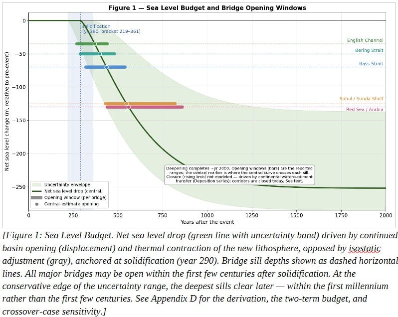The conclusion holds across the parameter range, and it no longer depends on the two terms rescuing each other. Thermal contraction alone delivers 272 m of gross drop — 190 m net — which clears the deepest controlling depth in the table (Sunda, 125 m) without any contribution from continued separation. The deepest sill clears by year 731 even on the slow solidification anchor. Moving any single parameter to its conservative end still clears it with more than 70 m to spare. The largest excursion is not the shallow mechanical basin depth but the severe profile assignment — putting the whole of Appendix F's ±16% band on the removed/retained split — which leaves a 196 m plateau against the 125 m sill. The softest assumption runs the conservative way: the thermal term is computed at the free-shrinkage strain mode, and a laterally confined column would contract vertically by roughly a factor of three more, deepening the drop rather than reducing it — and the sills sit at the margins, which is where confinement is most likely to apply. The sensitivity of these results to the key uncertain parameters — the thermal contraction magnitude and the solidification timing — is analyzed in Appendix D. The conclusion holds: across the plausible range, all major land bridges open within the first few centuries to the first millennium after solidification. Even the largest single-parameter excursion — the severe profile assignment, on the slow anchor — clears the deepest sill inside the first millennium, at approximately year 800. Figure 1 shows the sea level budget over time, anchored at solidification (year 293–463). Continued basin opening and thermal contraction of the new lithosphere together drive the gross drop; the curve plotted is the net drop after the isostatic correction. It crosses each bridge's controlling depth between the first few centuries and the first millennium after solidification, the shallow straits leading and the broad shelves trailing.

[Figure 1: Sea Level Budget. Net sea level drop after isostatic correction (green line, with an envelope spanning single-parameter excursions) driven by continued basin opening (displacement) and thermal contraction of the new lithosphere, anchored at solidification (year 293–463). Bridge sill depths shown as dashed horizontal lines. Every major bridge opens within the first few centuries to the first millennium after solidification, the shallow straits leading and the broad shelves trailing. Ice is omitted from the curve; including it moves every crossing earlier. Bars are the opening windows across the solidification bracket; markers are where the reference curve crosses each depth. See Appendix D for the derivation, the two-term budget, and the parameter sensitivity.]

When the Bridges Open

The sea level budget translates directly into land bridge timing. Each bridge opens when the net sea level drop exceeds the sill depth of the strait. The shallowest sills clear first, the deepest last, as the floor continues to deepen through the first few centuries after solidification.

Windows span the boiling-flux crossover bracket — solidification at year 293 for the fast case and year 463 for the slow one — at the 20,000 km rift and 0.8 km mechanical depth throughout. The short rift is the conservative case: a longer one only adds displacement and moves every window earlier. Where a bridge is a broad shelf rather than a narrow strait, the stated sill range is the depth span of the shelf, not an uncertainty in a single sill; the controlling depth is the point past which the crossing is continuously passable, and it is that depth the window is computed at. Sunda is the clearest case: the shelf carries 2.5 M km² of exposed ground long before its deepest point is dry, and waiting for 200 m would misstate when the corridor is walkable. Parameter uncertainty is treated separately in Appendix D, one parameter at a time; no single conservative excursion prevents any of these bridges from opening. These windows also omit any contribution from ice, which would move every date earlier — see Appendix D. Every major intercontinental bridge opens within roughly the first few centuries to the first millennium after lithosphere forms — the shallow straits within about a century of solidification, the deepest within a few centuries more. Across the solidification bracket the openings fall between year 344 and year 731 from the event, with the shallow bridges leading and the deep bridges trailing. The corridors then remain open through a long connectivity window before closing. The closing is treated separately and with less precision than the opening, for a reason grounded in the physics. The opening is driven by basin deepening — continued spreading and thermal contraction — both of which are anchored on present-day observables and are essentially complete within the first few centuries. The closing is driven by the slower return of water to the deepened basins: the transfer of water and sediment off the continents and into the oceans, the mechanistic subject of the companion Deposition series, together with the redistribution of crustal load as the continents unload and the basins fill. These processes raise relative sea level at the sills and re-drown the corridors. Their timing and magnitude are not quantifiable from the observables used in this paper, so this paper does not assign closure dates. What is certain is the outcome: the corridors are closed today. Closure therefore happened — the only open question is its precise schedule, which the present model does not predict. The dispersal window is best characterized as opening within the first few centuries after solidification and remaining open for centuries thereafter, closing gradually as the continents shed their water and sediment into the basins.

The Corridors

Climate Shapes the Highway

A land bridge is not a highway unless it has food. The climate profile at each corridor determines which animals can use it, because the climate determines what grows there. Because every corridor is ultimately fed by the same warm-ocean moisture source and volcanic aerosol cooling, the primary differences among them arise from latitude, distance from the coast, and local topography. Seven major corridors radiate from the landing zone in the Armenian Highlands: the Eurasian Highland trunk (35–50°N), Beringia (60–70°N), the Sunda Shelf (0–10°S), the Sahul Shelf (0–40°S), the Arabian/Red Sea corridor (15–30°N), Doggerland (50–55°N), and the Bab el-Mandeb crossing. Each has a distinct climate character — temperature, precipitation, and coastal-to-inland moisture gradient — that acts as an environmental filter on the animals passing through. The Eurasian Highland (35–50°N) is the primary trunk. Every animal starts here. Warm temperate woodland — 14–23°C, 900–2,100 mm/yr precipitation — habitable in all directions from day one. No filtering. This is the launching pad. Beringia (60–70°N) is a cold filter. Tundra shrubland — temperatures below freezing year-round, 200–1,100 mm/yr. Passable but harsh. This corridor selects for cold-adapted megafauna: mammoth, bison, wolf, bear. Tropical species are excluded entirely. The Sunda Shelf (0–10°S) is a tropical superhighway. Dense rainforest — 26–31°C, 2,600–4,500 mm/yr. Minimal filtering. Everything that reaches this corridor gets through. The 2.5 million km² of exposed shelf at peak lowstand is the largest single expanse of newly available tropical habitat on the planet. The Sahul Shelf connects to Australia and New Guinea. Tropical at the entry (New Guinea), grading to warm temperate (Tasmania). The coastal corridor is dense rainforest; the interior opens to seasonal woodland. A long-lived bridge with moderate filtering — forest-adapted species travel the coast, grassland species follow later as the interior dries. The Arabian corridor (15–30°N) is the Africa filter — and the sharpest one. Coastal precipitation of 1,100–2,500 mm/yr drops to 100–600 mm/yr within a few hundred kilometers inland. A narrow humid coastal strip with desert immediately behind it. This corridor selects for large, mobile species capable of traversing semi-arid gaps: elephants, big cats, bovids. Small forest-dependent species requiring continuous dense cover are excluded. This filtering explains why Africa's founding fauna is dominated by large mammals rather than small forest specialists. Doggerland (50–55°N) extends the Eurasian trunk westward, connecting Britain to continental Europe. Cool temperate throughout. Minimal filtering. The Bab el-Mandeb crossing at the southern end of the Red Sea provides a second, narrower connection to Africa. Climate and filtering character are similar to the Arabian corridor — a thin productive coastal strip with arid interior — but the crossing itself is shorter and more direct. The precipitation gradient — not the temperature gradient — is the dominant control on corridor character. Coastal zones typically receive 2–5 times the annual precipitation of interior zones at the same latitude, creating lush coastal highways bordered by progressively drier woodlands and steppe. The moisture comes from the warm ocean; the gradient comes from distance. Animals following coastal corridors walk through lush habitat. Those attempting interior crossings face progressively drier conditions. The extreme precipitation also rebuilds the freshwater system that animals require for survival. Fresh water is less dense than salt water and floats. Highland streams run fresh from the moment rain hits exposed rock — the water has never contacted the ocean. At 2–4 times modern precipitation rates, freshwater lenses form on the surface of any standing water within days, enclosed basins flush from saline to fresh within months, and rivers carve new channels fed entirely by rainfall. By the time the land bridges open and animals begin to disperse, every corridor has functioning freshwater drainage — streams, rivers, pools, and lakes — established from the highlands downward by months to years of extreme rainfall. The full corridor climate profiles, developed independently of the energy balance model, are presented in Appendix E.

The Table Is Set

Vegetation Leads the Animals

A corridor with the right climate is still impassable if nothing grows there. The critical question is whether vegetation establishes fast enough on post-catastrophe terrain to support animal populations within the bridge windows. The published literature on volcanic succession answers this unambiguously: yes. Krakatoa, sterilized to bare rock in 1883, supported dense grassland within three years, woodland within fifty, and mature tropical forest within a century. Mount St. Helens, devastated in 1980, showed pioneer vegetation within months — fireweed, grasses, and lupines — with visible forest recovery within fifteen years. These are cases of primary succession, starting from nothing: no surviving roots, no seed bank, no soil biology. Seeds arrived by wind and water from distant sources across open ocean or devastated terrain. The post-catastrophe landscape in this model does not start from nothing. The brief, dynamic inundation described in the first paper (Proposition 3) leaves surviving root systems, seed banks, and soil microbiomes. This is secondary succession, which the ecological literature consistently shows is 5–10 times faster than primary succession. The Genesis text provides a direct data point confirming this timeline. At day 272 — approximately seven months after the onset and months after the highlands first emerged — the dove returns carrying a freshly plucked olive leaf. As established in the first paper (Proposition 6), olive trees survive brief saltwater inundation and resprout vigorously on volcanic ash soil under heavy rainfall. The olive leaf is not a miracle. It is a field measurement confirming that secondary succession on the highlands is already months old — consistent with the published recovery rates from Krakatoa and Mount St. Helens, and likely faster given the surviving root systems and extreme precipitation. Three additional factors accelerate the process beyond what modern analogs demonstrate. First, precipitation runs at 2–4 times modern rates, accelerating every stage of the succession cycle — salt washout, germination, nutrient cycling, and growth. Second, continuous volcanic ash deposition provides an ongoing supply of mineral nutrients. Published research shows that volcanic ash at concentrations above 3% in soil triples plant biomass and restructures the soil microbiome to promote plant-growth-promoting bacteria — the soil ecosystem, in the words of one research team, "flips a switch." Third, warm year-round temperatures in the tropical and subtropical corridors eliminate the cold-season growth limitation that slows succession at higher latitudes. The published data support specific timelines. At Krakatoa (primary succession on sterilized rock), grassland dominated within 14 years and closed-canopy tropical forest developed within a century. At Mount St. Helens (mixed primary and secondary succession), pioneer species appeared within months in areas with surviving root systems, plant cover reached 38% within 14 years and 66% within 20 years, and visible forest recovery occurred within 15 years. Under the more favorable conditions in this model — secondary succession with surviving root systems, 2–4× modern precipitation, and continuous volcanic ash fertilization — succession timelines are estimated at 5–10× faster than the primary succession observed at these sites. Scaling observed secondary succession rates by the three accelerating factors yields the following corridor-by-corridor estimates:

Vegetation timelines scaled from Krakatoa and Mount St. Helens secondary succession data, adjusted for 2–4× precipitation, continuous volcanic ash fertilization, and surviving root systems (5–10× acceleration over primary succession). Bridge windows are the ones derived above, on the same solidification bracket; Sunda and Sahul are listed separately because they do not open together — Sahul clears roughly forty years before Sunda, so the Sunda–Sahul corridor is walkable only from Sunda's date. In every corridor the vegetation timeline is shorter than the bridge window, so the bridge is what gates arrival throughout. The table is set before the guests arrive. Because the bridges open later — after lithosphere forms and the basins contract — the vegetation has even more time to establish. In every corridor, the animals walk into an ecosystem that is already growing, already producing food, and getting more productive every year. The delay in bridge opening, far from being a problem, widens the margin by which the food supply precedes the travelers.

Summary

The waters parted early. The new ocean basins form solid lithosphere at the latent-heat phase transition, bracketed at year 293–463 after the catastrophe. Only then does the floor begin to cool, contract, and subside, drawing sea level down. Within the first few centuries of solidification — by year 731 even on the slow anchor — the net drop clears every major intercontinental sill, and all the land bridges are open. The deepening that opens them comes from two sources acting together: cooling-contraction of the newly solidified floor, which is the larger, and continued separation of the continents opening new basin volume. The corridors remain open for centuries, then close gradually as the continents shed their water and sediment into the basins — a slower process whose schedule this paper does not predict, bounded by the certainty that the corridors are closed today. The opening timing carries a bracket of roughly +50 to −75 years from the uncertainty in the solidification date. These bridges are not barren rock. They are corridors shaped by a distinct climate — warm tropics driving massive evaporation, cold high latitudes building ice, and a steep coastal-to-inland precipitation gradient creating lush coastal highways flanked by drier interiors. Each corridor's climate acts as an environmental filter, admitting certain animals and excluding others. The vegetation is already there when the bridges open. Post-catastrophe succession, accelerated by extreme rainfall, volcanic ash fertilization, and surviving root systems, produces functional ecosystems in years to decades — faster than the bridges form. The system is a single machine. One equation — the plate velocity as a function of time — drives the schedule of everything: the ocean heating, the basin deepening, the mountain building, the volcanic forcing, the ice accumulation, the sea level drop, and the opening of the corridors. The magnitudes come from that same curve except for the thermal contraction, whose size is fixed by the measured heat flux and whose timing is not. Two primary observational constraints plus the narrative's recorded phase transition drive five major outputs. The animals exit the ark into a greening continent. The highways open within the first few centuries after the new sea floor solidifies. The vegetation is waiting for them. The question that remains — which animals walk which corridors, how fast they spread, and why each continent ends up with the fauna it has — is the subject of the final paper in this series.

What This Paper Does Not Claim

This paper does not claim to quantify ice volume or rate of ice accumulation. The energy balance model produces a temperature response to a calibrated forcing; it does not include ice sheet dynamics, ice-albedo positive feedback beyond the EBM's parameterization, or any mechanism for tracking ice mass. The conditions for ice accumulation — sustained polar cooling and enhanced moisture supply — are produced by the model. The resulting ice volume is not. A full ice sheet model would be required. The energy balance model is used solely as an indicative consistency check that the implied forcing yields a sane climate response. It does not predict absolute temperatures (its tropical values are artifacts of a simple EBM without convective limiting), the latitudinal pattern of cooling, the timing of return to modern climate (set by the model's heat capacity, not the scenario), or ice volume. This paper does not claim to model the spatial distribution of ocean surface temperature. The three-basin thermal architecture established in the Trigger Standalone — hot Atlantic and Indian rift basins, cool Pacific remnant — is a key feature of the post-catastrophe ocean, but is not simulated here. The downstream analysis (sea level budget, bridge timing) does not depend on basin-resolved SST. Readers interested in the basin-resolved heat budget are referred to Appendix F of the Trigger Standalone. This paper does not claim that the cloud albedo forcing is calibrated. The magnitude (-6 W/m² peak) is a plausible estimate of the radiative effect of near-continuous cloud cover over the boiling rift basins. It is presented as a component of the climate forcing because it is physically expected, but its exact magnitude requires a cloud-resolving model that is beyond the scope of this paper. The qualitative conclusion — that the catastrophe drives sustained high-latitude cooling sufficient to initiate ice accumulation — is robust to substantial variation in the cloud forcing magnitude. This paper does not claim that the quantitative results are precise. The sea level budget and corridor climate profiles are order-of-magnitude estimates derived from calibrated but simplified models. A full general circulation model would refine these numbers — but the extreme and rapidly varying forcing conditions of the post-catastrophe environment sit outside the calibration range of standard GCMs, making a reduced-complexity approach both necessary and more appropriate at this stage. This paper does not claim a precise sea level curve or precise bridge-opening dates. The subsidence is derived from two terms — continued geometric basin opening and thermal contraction of the new lithosphere — anchored on the plate velocity, the modern floor depth, and the modern heat flux. The thermal term carries uncertainty from the expansion coefficient and the strain mode (a factor of up to three between the unconfined and confined limits; the conservative unconfined value is adopted), and the timing carries a bracket of roughly ±85 years from the solidification date (the boiling-flux crossover, years 293–463). The rift length that sets the basin geometry is carried as a bracket rather than a value; it scales the displacement term and does not enter the thermal one, which depends on heat removed per unit area rather than on how widely that heat is spread. The conclusion that all major bridges open within the first few centuries to the first millennium after solidification holds across the range, but the exact dates are not claimed. This paper does not predict sea level before the new ocean floor solidifies. Before the latent-heat phase transition (year 293–463), the basin floor is a transient, gas-charged melt body whose elevation is not constrainable from the available observables. The model is silent on sea level in that window by design. A brief early transgression — the squeezed Pacific rising while the new basins remain shallow — is physically expected there but is not quantified. The froth collapse of the solidifying melt body is likewise acknowledged as an additive contribution to the early drop but is not quantified. This paper does not predict when the land bridges close. The opening is driven by basin deepening, which is anchored on present-day observables and complete within the first few centuries. The closing is driven by the slower return of water and sediment from the continents to the basins — the mechanistic subject of the companion Deposition series — and by the associated redistribution of crustal load. The timing and magnitude of closure are not constrainable from the observables used in this paper, so no closure dates are assigned. The outcome is nonetheless certain from direct observation: the corridors are closed today. The paper therefore states that the corridors open within the first few centuries after solidification and close gradually thereafter, without assigning the closure a date. This paper does not claim that the vegetation succession timeline is precisely calibrated to the post-catastrophe conditions. The modern volcanic analogs (Krakatoa, Mount St. Helens, Surtsey) provide directional evidence and order-of-magnitude timing, but no modern event matches the scale, precipitation intensity, or biological starting conditions of the model. The claim is that vegetation establishes faster in this model than in the observed analogs, not that the exact timeline is known. This paper does not claim that the corridor climate profiles represent exact conditions at any specific location. They are latitude-band averages with coastal-inland gradients, derived from an energy balance model and independently validated. Local topography, ocean currents, and regional weather patterns would modify these profiles substantially. The claim is that the corridors are habitable, not that their precise temperature and precipitation at any given point are known. This paper does not address the biological response — which animals use which corridors, how fast they spread, or why each continent's fauna looks the way it does. That is the subject of the companion paper. This paper does not claim that the Genesis narrative is independently verified. What it does claim is that the velocity model takes no parameter from the text — not a date, not a duration, not a rate. The narrative supplies the shape of the event, a violent onset followed by decline, and the timing of an observation about the water at day 40; it sets nothing that is computed here. The physics is inherited from the foundational standalone and constrained by the observed continental separation. The framework should still be evaluated as an "if…then" proposition: if the account describes a real event, then these are the physical consequences — but the numbers do not come from the account.

Appendices

Appendix A: Plate Velocity

This paper does not derive a velocity model. It uses the one developed in the foundational standalone, "What Broke the Foundations?", and this appendix records what is taken and why it is usable here. What the specification contributes, and what it does not. The narrative records a violent initiation followed by a rapid decline — a change of character after a brief initial period, from mabbul to mayim. That is information about the shape of the event: a process that is severe at onset and then subsides, rather than one proceeding at a steady rate or building toward a peak. It is consistent with a decaying velocity profile, which is what the mechanism independently produces as the driving stress relaxes and the weakened pathways heal. The specification sets none of the parameters below. No date, no duration and no velocity is taken from the text. What is inherited. Phase 1 of the Trigger's velocity profile: v(t) = v_peak × exp(−t / τ₁), with v_peak ≈ 12 km/yr and τ₁ ≈ 417 years. Why τ₁ is determined without reference to elapsed time. The peak velocity comes from the forward physics model — cork-popping geometry, grain-size evolution, hydration and partial melt, each quantified from published experimental data. The total displacement comes from the observed continental separation, 5,000 km. Since the displacement delivered by the decay is τ₁ × (v_peak − v_crit), where v_crit ≈ 0.0267 km/yr is the speed at which the localized shear zones close — inherited from the Trigger, not derived here — the decay constant follows directly: 5,000 / (12 − 0.0267) ≈ 417.5 years. Both inputs are external to this framework's chronology, and no assumption about when the event occurred enters at any point. Scope of the inheritance. Phase 1 continues until the velocity decays to the critical value at which the localized shear zones close — at the reference peak, approximately year 2,550, though the crossing scales with τ₁ and runs from roughly year 2,000 at a 16 km/yr peak to year 4,000 at 7 km/yr. Every bridge date in this paper falls between the solidification of the new basin floor and roughly year 750, so the later phases of the Trigger's profile — and the healing timescale that governs them — are not used here and no result in this paper depends on them. Sensitivity. The uncertainty is the Trigger's own velocity envelope, v_peak from 7 to 16 km/yr, with τ₁ = 5,000 / v_peak in each case so that the observed separation is reproduced throughout. The envelope drops v_crit from the denominator used in the derivation above; across the whole range that changes τ₁ by less than half a percent, and every figure in the table below uses the simpler form. The quantity this paper consumes is displacement delivered after solidification, so it depends on the solidification anchor as well as on the peak. The anchor is itself a bracket — year 293 at the fast boiling flux, year 463 at the slow (Appendix D) — and both ends are shown:

The anchor matters more than the peak. Across the whole velocity envelope the spread is 11% at year 600 and 19% at year 1,000 on the fast anchor. Moving from the fast anchor to the slow one cuts the displacement delivered by year 600 by roughly a factor of three, because it removes 170 years from the front of the decay where most of the motion is. The peak velocity is the smaller uncertainty of the two, and the bridge timings in the main text inherit both. On the fast anchor the peak-velocity spread is not monotonic — a higher peak delivers more early and decays faster, a lower peak the reverse, and because v_peak × τ₁ is pinned by the observed separation the two effects largely offset. That offsetting weakens on the slow anchor and fails altogether by year 1,000, where the window sampled is late enough that the slow-peak cases have pulled clear: the spread widens to 16% at year 600 and 38% at year 1,000, and the year-1,000 column runs monotonically. The offset is a property of sampling the curve early, not a general one, and it is not relied on.

Appendix B: Climate Model Calibration and Catastrophist Run

This appendix documents the climate model setup, calibration, and limitations. The script reproducing the temperature results was written and run, but is not published and is not offered as citable work; what follows is a complete specification of what it does, which is what a reader would need to reproduce it. Model. The energy balance model used is climlab's EBM_annual (Rose, 2018), a one-dimensional annual-mean latitude-resolved energy balance model with diffusive heat transport, ice-albedo feedback, and a parameterized longwave radiation scheme (OLR = A + B·T). The model has 36 latitude bands from 87.5°S to 87.5°N. Calibration to modern climate. The model was calibrated to reproduce modern global mean temperature by tuning the OLR intercept parameter A:

The calibrated baseline produces a modern global mean temperature of 14.67°C, against an observed value of approximately 14.7°C. Sensitivity calibration. The model's equilibrium climate sensitivity is set by B = 2.0 W/m²/K, giving λ = 0.5 K/(W/m²). A sustained +4 W/m² forcing produces a 1.63°C equilibrium global cooling after 100 model years. That sensitivity sits at the low end of mainstream assessed values (IPCC 2021) rather than at their centre, which is the conservative direction here: a less sensitive model produces less cooling for the same forcing. No figure from that assessment is reproduced, and none is needed — the model is used only to show that the implied forcing gives a bounded response, not to assign a temperature. Limitation: transient volcanic response. The annual-mean EBM equilibrates each timestep and therefore cannot reproduce the transient peak cooling observed after individual volcanic eruptions such as Pinatubo (1991) and Tambora (1815), whose radiative forcing lasts months rather than centuries. Two figures circulate for Pinatubo's peak and they are not the same quantity: satellite radiometry measured a global forcing of about −2.7 W/m² in August 1991 (Minnis et al. 1993), the first unambiguous direct measurement of a climate forcing at that scale, while contemporaneous general-circulation modelling placed it nearer −4 W/m² at the tropopause (Hansen et al. 1992). The observed surface response was a global cooling of a few tenths of a degree, reflecting ocean thermal inertia and the brief duration of the forcing, neither of which the annual EBM captures. The validation run applies the −4 W/m² model value and returns 0.03 °C; that shortfall is the documented limitation rather than a defect in the calibration. For the catastrophist run, the forcings are sustained for centuries — well above the annual model's resolution — so the equilibrium response is the correct measure. The equilibrium sensitivity, not the transient response, is the calibration anchor.

Sources for this appendix.

• Rose, B. E. J. (2018). CLIMLAB: a Python toolkit for interactive, process-oriented climate modeling. Journal of Open Source Software, 3(24), 659. https://doi.org/10.21105/joss.00659

• Minnis, P., Harrison, E. F., Stowe, L. L., Gibson, G. G., Denn, F. M., Doelling, D. R., & Smith, W. L. (1993). Radiative climate forcing by the Mount Pinatubo eruption. Science, 259(5100), 1411–1415. https://doi.org/10.1126/science.259.5100.1411

• Hansen, J., Lacis, A., Ruedy, R., & Sato, M. (1992). Potential climate impact of Mount Pinatubo eruption. Geophysical Research Letters, 19(2), 215–218. https://doi.org/10.1029/91GL02788

• IPCC (2021). Climate Change 2021: The Physical Science Basis. Contribution of Working Group I to the Sixth Assessment Report. Cambridge University Press. https://doi.org/10.1017/9781009157896

Catastrophist forcing. Two time-varying forcings were applied: Volcanic. F_volcanic(t) = -6.0 × v(t) / v(0), where v(t) is the plate velocity inherited from the Trigger Standalone (Phase 1, v_peak = 12 km/yr, τ₁ = 417.5 yr). Peak: -6 W/m² at year 0; decays exponentially with plate velocity. Cloud albedo. F_cloud(t) = -6.0 × (f_earth(t) / 0.20), where f_earth(t) is the fraction of Earth's surface covered by the rift basins at time t. Peak: approximately -6 W/m² at full basin area. The run applies this forcing over years 0 to 800, and that window was set rather than derived. Appendix F of the Trigger Standalone places the end of boiling between year 603 and year 941 across the 10–20 kW/m² flux bracket, so 800 falls inside the bracket but runs past the two faster cases and short of the slowest. The forcing is also at full strength when it is switched off rather than tapering, which makes the choice of date a real one rather than a formality. Re-running the model with the cutoff at 603 and at 941 measures what that costs. Through the forcing period the answer is nothing: global mean temperature is identical to two decimal places at years 0, 100, 300 and 500 across all three cutoffs. The difference appears only in the recovery — up to 2.7 °C around year 750 and 1.1 °C at year 1,000 — and it has closed entirely by year 1,500. The cutoff therefore does not touch the cooling this paper draws on, and moves only the recovery date, which is one of the quantities the main text explicitly declines to assign. The forcings were applied additively to the OLR intercept: A_eff(t) = A + |F_volcanic(t) + F_cloud(t)|. Reduced volcanic forcing rationale. The -10 W/m² figure in earlier drafts of this paper assumed full eruption rate at approximately 75× modern with stratospheric injection. In the cork-pop mechanism, the majority of catastrophic eruption is submarine ridge volcanism, which has negligible radiative impact. The subaerial fraction (continental arc volcanism and flood basalt provinces) is the radiatively active component. With approximately 60% of the original reference value attributable to subaerial sources, the effective forcing reduces to approximately -6 W/m². This is an estimate, not a calibrated derivation. What this model does not produce. The model produces temperature response to radiative forcing. It does not produce ice sheet volume or accumulation rate (no ice sheet dynamics module), ocean SST distribution (no ocean basin geometry), precipitation patterns (no atmospheric moisture transport), or regional climate (zonal annual mean only). The sea level budget in this paper uses continued basin opening (pure geometry, no climate model required), thermal contraction of the solidified floor (from the heat budget in Appendix F of the Trigger Standalone), and isostatic adjustment (Airy correction at 30%). Neither the ice contribution nor the thermal expansion of the warming ocean is quantified; both are acknowledged as physically real and both are omitted from the budget, and they run in opposite directions.

Appendix C: Volcanic Forcing Derivation

The volcanic forcing applied in the catastrophist run is derived from three components: the eruption rate (set by plate velocity), the subaerial fraction of total eruption (the radiatively active component), and the washout physics that limits tropospheric aerosol residence time at high precipitation. A fourth quantity — the sulfur emitted by submarine basin emplacement — is treated here as well, but it is routed to the cloud-albedo term in the main text rather than to the stratospheric forcing derived below. Eruption rate. Plate velocity determines magma production at the spreading ridges, which in turn sets the SO₂ flux. At the inherited peak velocity (12 km/yr, from the Trigger Standalone), the integrated mid-ocean ridge eruption rate is approximately 75 times the modern global volcanic output. This is not a free parameter; it follows from the plate velocity that is in turn constrained by the observed continental separation. Subaerial fraction. The subaerial fraction — continental arc volcanism at the Ring of Fire and flood basalt provinces along separating margins — is the component that loads the upper atmosphere with sulfate aerosols and is the basis for the stratospheric forcing derived here. Modern ratio is approximately 25% subaerial / 75% submarine by volume. Under catastrophic conditions with explosive continental rifting, the subaerial fraction may be modestly higher (estimated 25–40%). The radiatively active eruption rate is therefore approximately 25–40% × 75× ≈ 19–30× modern. The submarine remainder is not radiatively inert — its disposition is treated under "Submarine basin sulfur" below — but it does not contribute to the stratospheric forcing computed in this appendix. Washout physics. The Seinfeld-Pandis aerosol scavenging coefficient λ = a × R^b (a = 5 × 10⁻⁵ s⁻¹, b = 0.7, R = precipitation rate in mm/hr) gives tropospheric aerosol residence times of approximately 0.3–0.4 days at the extreme post-catastrophe precipitation rates (12–15 mm/day). Tropospheric aerosols are scrubbed in hours; only the stratospheric fraction provides persistent radiative forcing. The stratospheric injection fraction from explosive subaerial eruption is approximately 10–30%. Submarine basin sulfur. The submarine fraction is conventionally dismissed as radiatively negligible, on the model of deep passive ridge volcanism: at mid-ocean-ridge depths the hydrostatic pressure suppresses volatile exsolution and any sulfur stays dissolved in the melt or the water column. That regime does not apply to the rift-basin emplacement in this model, which occurs at or near the surface against boiling seawater. Two sub-regimes operate, with opposite behavior. At a freshly opening margin, magma is driven up under pressure and makes direct contact with liquid water before a stable insulating vapor film can form; this is the explosive molten-fuel-coolant regime — rapid repeated flashing, fine fragmentation, and sulfur thrown clear of the melt before the surrounding brine can capture it. Once a steady vapor film establishes (the Leidenfrost regime), the film insulates the magma, the interaction quiets, and the boiling brine scrubs most of the exsolved SO₂ before it escapes. The violent regime is brief at any single point, but the margin advances continuously for centuries as the continents separate, so the explosive front is perpetually renewed along thousands of kilometers of opening rift; its intensity scales with plate velocity in the same way the ridge eruption rate does. The fate of this sulfur differs from the subaerial fraction: the plumes are Surtseyan, topping out in the upper troposphere (~9 km) rather than reaching the stratosphere, and what does reach the lower atmosphere is rained out within a day by the washout physics above. It therefore contributes essentially nothing to the persistent stratospheric forcing. Its significance is indirect — as sulfate, it is among the most effective cloud condensation nuclei known, and it seeds and brightens the basin cloud deck. It is accounted for in the cloud-albedo term in the main text, not here, and no part of it is added to the −6 W/m² figure below. Net forcing. Combining the subaerial fraction (≈ 30% central estimate), the stratospheric injection fraction (≈ 15% central estimate), and the logarithmic saturation of radiative forcing at high aerosol optical depth (F ≈ -25 × ln(1 + AOD)), the effective steady-state forcing is approximately -6 W/m² at peak velocity. Time dependence. The forcing decays exponentially with plate velocity: F_volcanic(t) = -6.0 × v(t) / v(0). This produces the volcanic-forcing values used in the main text. Sensitivity. Across the plausible range of subaerial fractions (25–40%) and stratospheric injection fractions (10–30%), the peak forcing ranges from approximately -4 to -8 W/m². The qualitative conclusion — sustained high-latitude cooling sufficient to initiate ice accumulation — holds across this range. The cloud albedo contribution discussed in the main text (estimated -6 W/m² peak) is independent of this volcanic forcing and provides additional cooling whose magnitude is similarly bracketed but less well constrained; the submarine basin sulfur described above strengthens the physical basis for that cloud term but does not change its estimated magnitude.

Appendix D: Basin Subsidence — Two-Term Deepening Model

The sea level drop in this model is driven by the deepening of the new ocean basins after their floors solidify. Two physical processes contribute: continued geometric opening of basin volume as the continents separate, and thermal contraction of the solidified floor as it cools. This appendix derives both, anchored on present-day observables, without invoking the conventional age-depth (√age) relation — which is calibrated in millions of years and would import the deep-time assumption this framework rejects. Why not the √age curve. The conventional ocean-floor subsidence relation, d(t) = d_ridge + C·√(age), describes incremental crust accreted strip-by-strip at a spreading ridge, each strip cooling from its own formation moment. The new basins in this model do not form that way. The floor is emplaced as a single hot, gas-charged melt body that loses latent heat through the boiling discharge and then solidifies near-batch at the phase transition. The relevant physics is bulk cooling of a solidified volume plus continued geometric basin opening, not strip accretion. The √age coefficient and its Myr calibration do not apply. Term 1 — Displacement (geometric). As the continents continue to separate after the floor solidifies, new basin volume opens at a rate set by the plate velocity. This is a purely geometric effect: an added slot of basin volume, rift length × mechanical basin depth × incremental separation, and the ocean surface falls as that slot opens beneath it. The mechanical depth here is the 0.5–1.0 km over which the opening translates into basin capacity — a different and much smaller quantity than the emplaced thermal column, and the two are not to be conflated. The conversion is the basin cross-section divided by the ocean area — rift length × mechanical basin depth ÷ 3.6 × 10¹⁴ m² — which at the 0.8 km reference depth gives 0.044 m of gross drop per kilometer of post-solidification displacement at a rift length of 20,000 km, and 0.080 m/km at 36,000 km. Integrating the velocity profile forward from solidification, the displacement-driven gross drop at completion is 72–109 m at a 20,000 km rift and 129–195 m at 36,000 km, the range within each set by where in the solidification bracket the clock starts. This term carries no thermal assumptions; its inputs are the plate velocity, the mechanical basin depth (bracketed 0.5–1.0 km), and the rift length (bracketed 20,000–36,000 km).

Term 2 — Thermal contraction, from the heat budget. Once the column solidifies it cools toward the modern geotherm and contracts. The contraction of a cooling column is

Δd = α_eff · ∫ ΔT(z) dz

and this appendix does not evaluate that integral from an assumed thickness and an assumed mean temperature. It takes it from the energy, because the sensible heat removed per unit area is the same integral multiplied by the material properties:

E_sensible / A = ρ c ∫ ΔT(z) dz

so that

Δd = α_eff · (E_sensible / A) / (ρ c)

The column thickness cancels, and so does the shape of the temperature profile. This matters because neither is known. The foundational standalone's Appendix F states plainly that its 57.6 km column is "the thickness of the equivalent linear column, not an observed lid," that the real body's internal temperature profile is not known, and that the depth at which solid gives way to melt within it is not known either. Neither enters the conversion. A subsidence derived this way therefore requires no lithospheric thickness and no emplaced volume, and the shape of the profile drops out of the arithmetic that turns heat into contraction. The profile does still bear on how much sensible heat has been removed, which is the quantity fed in, and that dependence is carried explicitly further down rather than claimed away here. What counts and what does not. Only sensible heat removed below the solidus drives thermal contraction. Latent heat is a phase change with its own volume coefficient and is excluded; crystallization shrinkage is a separate effect not carried in this term. Sensible heat removed above the solidus is also excluded, because that material has not yet solidified. Appendix F's per-cubic-meter decomposition separates them:

The present thermal profile runs from 2 °C at the sea floor to the solidus at the base of the solidified column, so its mean sits at the midpoint of that range. Exactly half the sub-solidus sensible heat has therefore left, and exactly half remains in the ground — which makes the heat that drove the contraction identical to the heat still retained:

E_sensible,removed  =  E_retained  =  8.76 × 10²⁷ J

The equality is exact given that linear form, and it reproduces the figure Appendix F publishes for its retained term. But the linear profile is Appendix F's equivalence, not an observation: F states that the real interior profile is not known and prices the uncertainty at ±16% on delivered energy. The pin above is therefore the linear-equivalent pin, and a resolved profile would move it — bottom-weighted leaves more heat in the ground and shrinks this term, top-weighted does the reverse. That sensitivity is carried explicitly below rather than absorbed. What does not move is the identity itself, which holds for any profile. The result. Over the 10⁸ km² of new basin:

E_sensible / A  =  8.76 × 10¹³ J/m²
∫ ΔT dz        =  3.02 × 10⁷ K·m
Δd_thermal     =  272 m gross,  190 m net

The strain-mode choice (α_eff) is the only free quantity remaining in this term. Its value depends on how the cooling column is mechanically constrained. A laterally confined column directs all its thermal contraction into vertical subsidence and takes the full volumetric coefficient (α_vol ≈ 2.7 × 10⁻⁵ K⁻¹). A laterally unconfined column shrinks in all three dimensions and takes the linear coefficient (α_vol / 3 ≈ 9 × 10⁻⁶ K⁻¹). The basin geometry determines which applies. At solidification the basin is already some 2,500 km wide on each flank of the rift and is still widening; the newly solidified floor is bordered by mush and open water, not by rigid confining lithosphere, and the continental margins are receding. The floor is therefore laterally unconfined for the prediction-relevant interval, and the linear coefficient is adopted. This is the conservative choice — it yields the smaller thermal drop. The confined limit would roughly triple this term; it is noted as an upper bound and not adopted, because the geometry does not support it across the basin as a whole. One asymmetry is worth naming: the sills sit at the margins, where the new floor abuts continental crust, and that is precisely where lateral confinement is most likely to apply. If it does, the drop at the sills exceeds the basin-mean value used here. The unconfined coefficient is adopted throughout regardless, so any margin confinement only adds to the margin already reported.

The solidification anchor. Contraction begins when the body drops below the solidus, which the release history determines rather than a separate assumption. Appendix F's Phase 1→2 crossing gives:

All timing below is stated from that anchor, and the bracket year 293–463 is the source of the opening window quoted for each bridge in the main text. The timing. Both terms are front-loaded. The displacement term follows the decaying plate velocity. The thermal term follows the sub-solidus portion of the boiling discharge, taken from Appendix F's release history and pinned to the 8.76 × 10²⁷ J total. Reference geometry, 20,000 km rift at 0.8 km mechanical depth, ice-free:

Net drop at the margins. The gross deepening is reduced at the continental margins by the isostatic correction (standard Airy correction, ≈ 30% of gross). The net drop available to clear the bridge sills is therefore approximately 0.70 × gross, reaching 240–327 m at completion across the solidification bracket and the rift-length bracket together. Opening windows. Ice-free, at the 20,000 km rift and 0.8 km mechanical depth, windows spanning the fast anchor to the slow. The short rift is the conservative case for these dates: a longer rift only adds Term 1 and moves every window earlier.

Every sill clears on basin deepening alone, with no ice contribution required.

The rift-length bracket applies to Term 1 only. Term 2 depends on the heat removed per unit area, which does not change with how widely that heat is spread — a longer rift opens a wider basin but delivers proportionally more energy into it, and the two scale together. Only Term 1 varies with rift length. The total net drop across the bracket runs 241–266 m at 20,000 km and 281–327 m at 36,000 km. The bracket ends have different provenance and the paper does not choose between them. The low end is the rift length the foundational standalone states. The high end sums the modern ridge systems the new basins correspond to. Whether an effective model rift length and a traced modern ridge length are the same quantity is a question a three-dimensional treatment would settle; this paper's conclusion does not require the answer. Robustness. The conclusion does not rest on a cancellation between the two terms. Term 2 is 272 m gross on its own, which clears every sill in the table at the reference correction without any contribution from Term 1. Taking the slow solidification case and moving one parameter at a time against the deepest sill:

The profile rows apply Appendix F's ±16% band on delivered energy to the removed/retained split in full: 8.76 × 10²⁷ ± 0.16 × 1.795 × 10²⁸ J, giving 5.89–11.63 × 10²⁷ J and a Term 2 of 183–361 m gross against 272 m at the linear case. Assigning the whole of F's band to this one split is the severe reading — the band is quoted on delivered energy, not on the split — and it is used here because it brackets the term rather than tuning it. Every row shares the same baseline: 27,000 km rift, 0.8 km mechanical depth, slow anchor, Term 1 = 97 m gross. Every excursion clears the deepest sill, and the smallest margin among them is 71 m. The parameters are tested singly because that is what the evidence supports: they are independent, and a combination driven to several conservative ends at once has no particular claim to being the governing case. Nothing here suggests they move together. The softest input is the strain-mode choice, and it is taken at its conservative value. Ice: an omitted term that runs one way. The budget above omits ice, and the omission is deliberate — this paper models no ice-sheet dynamics and predicts no ice volume. The ice-free budget is the conservative case, and every date above is a late one. The ice-age excess — the ice present at glacial maximum and since lost — is taken at the low end of conventional Last Glacial Maximum estimates, approximately 45 × 10⁶ km³, and this framework requires the whole of it to be post-event (Dating Capstone, Appendix A). That volume is 115 m of sea-level equivalent, and nothing in this paper is free to adjust it. The direction is not in doubt and is the only direction available: ice can only lower sea level while it is accumulating, so its effect is to open every bridge earlier and to leave the ordering unchanged. The magnitude over the opening window depends on the accumulation shape rather than on the volume, and this appendix does not derive that shape. No quantified ice case is therefore offered. The accumulation is limited by the boiling engine rather than by water availability — the companion appendix reports that the post-event moisture supply exceeds what the ice demands by one to two orders of magnitude — so the shape follows the thermal history and would have to be derived from it. That derivation is not attempted here. None of this is carried into the budget or the opening windows, which remain the ice-free case throughout. It is stated so that the conservatism is visible rather than silent. Additional unquantified contribution. As the gas-charged melt body solidifies, it also collapses from any elevated "froth" stand (vesiculation and active convection bulk up the agitated column; this collapses as the system degasses and settles). This adds to the early drop. Its magnitude depends on volatile content and emplacement conditions that are not constrainable from the available observables, so it is acknowledged but not quantified. It acts in the same direction as the other two terms. Closure. This paper predicts when the bridges open but not when they close. The opening mechanisms are front-loaded and largely complete within a few centuries: the displacement term follows the rapidly decaying plate velocity, and the thermal contraction follows the front-loaded boiling discharge. The closing mechanisms, by contrast, are cumulative and ongoing over much longer timescales — the transfer of water and sediment off the continents and into the oceans (the mechanistic subject of the companion Deposition series), together with the redistribution of crustal load as the continents unload and the basins fill. Because the opening is fast and the closing is slow and cumulative, the corridors stand open for a long window after the deepening completes. The closing processes' timing and magnitude are not constrainable from the observables used here, so no closure dates are assigned. The outcome, however, is fixed by direct observation: the corridors are closed today. Closure therefore occurred; only its schedule is unpredicted. This asymmetry — a well-constrained opening and an observationally-bounded but unquantified closing — is intrinsic to the available evidence and is stated rather than papered over. Methodological boundary. No sea level prediction is made before solidification. Before the phase transition, the floor is a transient melt body whose elevation is not constrainable. The first defensible point is at solidification, bracketed at year 293–463, and all timing is stated from that anchor.

Appendix E: Corridor Climate Profiles

Full latitude-by-time climate tables with coastal-inland precipitation gradients were derived for all seven corridors: Eurasian Highland, Beringia, Sunda, Sahul, Arabian, Bab el-Mandeb and Doggerland. They are not published and are not offered as citable work. They were derived independently of the energy balance model, and no comparison between the two is made here. The model is used in this paper in a proxy configuration only, as an indicative check that the implied forcing produces a bounded response; it assigns no latitudinal pattern and no absolute temperature, so there is nothing in it to validate these profiles against. What the profiles supply is qualitative character — hot tropics, cold poles, habitable mid-latitudes, and a coastal-inland precipitation gradient sharp enough to act as a filter on what moves through. That is what the corridor argument in the main text uses, and it does not depend on any temperature the model assigns.

← Where Did the Dove Find Peace? | Diaspora Series | Where Did the Kinds Walk? →

© 2026 D. L. White. Licensed under CC BY-ND 4.0. https://creativecommons.org/licenses/by-nd/4.0/ This paper was developed collaboratively using Claude (Anthropic) for technical modeling, calculations, and co-development of the reasoning chain. Earlier qualitative climate profiles were independently derived by Grok (xAI). The energy balance model was implemented in climlab (Rose, 2018), calibrated to modern global mean temperature (A=193, D=0.7, B=2.0), and driven with volcanic aerosol forcing and an estimated cloud albedo forcing tied to the velocity profile. Neither AI system endorses all conclusions as settled.