How Many Were There?
Most of a founding pair's variation is sorted within thirteen generations. How many such pairs it takes to produce the species alive today. Part Three of the Diversification Series.
How Many Were There?
The Drift Ceiling and the Kind Count
Part Three of the Diversification Series
The Question the Wolves Raised
The second paper in this series established two things about genetic diversity. It runs downhill, without exception, in every family examined. And the molecular clock — tested against a dog breed with a documented founding date — overestimates elapsed time by hundreds to thousands of times. It closed by asking: how many genetically distinct founding kinds does it take to produce the full roster of species alive today? And does that number fit inside anything that floats?
This paper answers both questions. But first, it must resolve a prior one: where does one ancestor end and another begin? If wolves and coyotes diversified from a common canid ancestor, and horses and donkeys from a common equid ancestor, how do we know the canid ancestor and the equid ancestor were different starting points rather than branches of an even deeper common ancestor?
This is the "kind" boundary problem. Creation scientists have been working on it for decades under the name baraminology, using hybridization data, visual similarity, and statistical trait analysis. Their results have been productive — roughly 137 mammalian kinds and 196 bird kinds by the most recent comprehensive estimates. But the methods are observational. They describe where the boundaries appear to fall. What they cannot supply is a quantity to test a grouping against — a figure, computed rather than observed, for how much divergence a single starting point could produce.
The drift model from the companion paper answers it from the other direction, and it answers it by calculation. Run the model forward from a single founding pair over the time available and it says how much genetic distance drift can open up between the descendants of one starting point. Any two populations separated by less than that could have come from one founding pair. Two populations separated by more could not, whatever a taxonomist has called them.
That is the whole test, and everything it needs is computed here. The order matters, so it is stated plainly: the calculation comes first, the measured families are tested against it, the count follows from which families pass, and the comparison with mainstream hybridization data arrives at the end — where it serves as a check on a result already in hand rather than as a premise the argument leans on.
What a Founding Pair Can Do
This series takes its window from the private mutational load calculation set out in the companion paper: two directly measured quantities, divided one by the other, with no assumed population size anywhere in it. That calculation places the founding point between 4,725 and 7,200 years ago, with a central value of 5,786. The work below runs at the central value and reports what the bounds do to it.
The drift equation that governs genetic differentiation between isolated populations is:
FST(t) = 1 − (1 − 1/(2Nₑ))^t
where Nₑ is the effective population size (roughly, the number of breeding individuals averaged over a population's history — typically much smaller than the total headcount) and t is the number of generations since the populations separated. At the central value of the window the generation count depends on the generation time: roughly 1,929 for canids (3-year generations), 1,157 for bovids (5-year), and 723 for equids (8-year).
A founding kind does not begin at some steady effective population size and stay there. It begins as a pair and grows. Modeling it that way — a pair, geometric growth, and a ceiling where the environment stops it — changes what the equation says, because the earliest generations do nearly all of the work. A pair doubling each generation accumulates an FST of 0.42 within about thirteen generations, and that figure is fixed regardless of how large the population eventually becomes. The per-generation drift terms sum to a converging series: a quarter, then an eighth, then a sixteenth. Almost all of the sorting is finished before the lineage has a hundred members in it.
What happens after that depends on the ceiling. A lineage that keeps expanding drifts more and more slowly, because drift weakens as population grows; a lineage that stops early keeps drifting at whatever size it stopped at.
Differentiation reached in 5,786 years, by population ceiling:
| Population ceiling | Canid (3-yr) | Bovid (5-yr) | Equid (8-yr) |
|---|---|---|---|
| 200 | 1.00 | 0.97 | 0.90 |
| 500 | 0.92 | 0.82 | 0.72 |
| 1,000 | 0.78 | 0.67 | 0.60 |
| 5,000 | 0.52 | 0.48 | 0.46 |
| 20,000 | 0.45 | 0.44 | 0.43 |
| 100,000 | 0.43 | 0.43 | 0.42 |
Growth is set at a doubling per generation, which is conservative for animals expanding into empty range — a canid pair with a litter of four clears it easily, and a mare produces roughly eight foals in an eight-year generation. Varying it from twice to eight times moves the two-hundred-ceiling row by no more than 0.02, from 1.00, 0.97 and 0.90 at a doubling to 0.99, 0.96 and 0.88 at eightfold, and leaves the large-ceiling rows between 0.28 and 0.43. Below a doubling the distinction blurs, and at 1.25× even a hundred-thousand-strong lineage reaches 0.74.
The window moves the figures less than the growth rate does. The table is computed at the central value of 5,786 years. At the lower bound of 4,725 the thousand-ceiling row reads 0.74, 0.64 and 0.57 instead of 0.78, 0.67 and 0.60, and the two-hundred-ceiling row stays between 0.87 and 0.99. Even at 4,000 years — below the window entirely — it reads 0.70, 0.61 and 0.55. Shortening the window moves the numbers. It does not move the pattern.
The model therefore does not produce a single figure. It produces a curve controlled by ceiling size: a lineage confined to a valley, an island, or a contracting range keeps rising well past 0.43, while a lineage that expanded into a large connected population plateaus there and effectively stops. The whole surface is printed above rather than a preferred row, and every ceiling from two hundred to a hundred thousand is computed at the same growth rate and the same window.
The floor of that surface is what the rest of this paper uses, because it is the hardest figure for a single-pair origin to clear. A lineage that expanded without limit — the case that produces the least differentiation the model can deliver — reaches roughly 0.43 and goes no further. That is the strictest reading of what one founding pair can do. Testing against it rather than against the maximum matters: the maximum is not a bar at all, since a tightly held lineage reaches 1.00 and would accommodate any observation whatsoever. A test that cannot fail establishes nothing. The floor can fail, and what follows is a test against the floor.
What the Model Assumes
Population size cannot be arbitrarily small. Modern conservation biology places the minimum viable population — the floor below which inbreeding and demographic bad luck threaten a lineage with extinction — at roughly 50 effective breeders.
The analysis throughout this series uses deliberately conservative parameters: an effective population floor of Ne = 50, and a starting heterozygosity of H₀ ≈ 0.40 to 0.50. Both understate the actual founding condition.
The modern minimum-viable-population figure of 50 exists because modern populations carry thousands of generations of accumulated copying errors — deleterious recessives that turn lethal when inbreeding exposes them. A founding pair with an undegraded genome carries no such load. Inbreeding between two maximally heterozygous, error-free individuals produces no inbreeding depression, because there are no hidden lethals to expose. The real floor for a pristine founding pair is not fifty. It is one pair.
That single pair is also more diverse than the model assumes. Two diploid individuals can carry up to four distinct alleles at every locus. A fully heterozygous founding pair with non-overlapping alleles has an expected heterozygosity near 0.75 — well above the 0.40 to 0.50 the model uses. Every parameter in the analysis therefore has room to spare in both directions: smaller founding populations drift faster, and a richer starting genome supplies more to sort. The conservative numbers were kept throughout not because they are accurate but because winning on the skeptic's assumptions is stronger than winning on one's own.
A four-allele ceiling per locus invites an obvious objection: can so few alleles account for the diversity observed across all the descendants of a kind? The objection conflates two different quantities. Four alleles is a ceiling on per-locus variety. It is not a ceiling on genome-wide variety, because a genome's distinct states are the combinations of its per-locus genotypes across many thousands of variable loci — and combinations multiply. Four alleles at a single locus yield ten possible genotypes. Across even a thousand independently varying loci, the number of distinct genome-wide states is on the order of ten raised to the thousandth power — a figure that dwarfs the number of individuals a kind has ever contained, by hundreds of orders of magnitude. The founding pair is not a narrow gate. It is a compact seed whose combinatorial unfolding vastly exceeds anything its descendants could exhaust. Recombination does not need many alleles to generate effectively unlimited genotypic variety. It needs a few, sorted across a large genome — which is exactly what a single undegraded pair provides.
Even so, very small founding populations remain subject to demographic stochasticity regardless of genome quality — random fluctuations in births, deaths, and sex ratios can end a lineage through sheer bad luck, and slow-breeding kinds are more exposed to it than fast-breeding ones. Some founding kinds may have been lost this way, which means the original kind count may have been slightly higher than what the modern species roster implies.
The initial small population size is not otherwise the liability it would be for a modern bottleneck. With empty ecological niches and no competition, population growth is explosive. Within a dozen generations, effective population sizes reach hundreds, then thousands. The early rapid drift at small Ne is precisely the mechanism that sorts the original variation into distinct lineages quickly — it is the engine of diversification, not a threat to it. The initial bottleneck drives speciation rather than endangering it.
Testing Families Against It
The test is now fixed and it is the paper's own: a taxonomic family is one kind if its most divergent within-family pair sits at or below roughly 0.43, the least differentiation a single founding pair can deliver over the window. A family whose internal distances exceeded that could not have come from one pair. It would not be one kind — it would have to be split, and the kind count would rise.
A methodological note before the figures. The bar was computed from the drift equation, the founding pair, the growth rate and the window. It was not fitted to any of the values below, which are independent published measurements. This is an out-of-sample check.
Within-family FST values, against a bar of 0.43:
Wolf–Coyote: FST ~0.40. These are the most divergent members of the canid kind. Passes, and it is the tightest case in the set — three hundredths under the bar. They still hybridize where their ranges overlap, which is what the model expects of two lineages that both expanded into continental populations.
Italian wolves vs Iberian wolves: FST = 0.293. Same kind, same species, different populations. Passes.
Dog vs Wolf: FST = 0.165. Passes.
Horse breed maximum (Clydesdale vs Mangalarga Paulista): FST = 0.254. Passes.
Cattle breed global average: FST = 0.100. Passes.
Human populations, most distant pairs: FST = 0.05 to 0.15, clustering at 0.05 to 0.10 for modern genome-wide estimates (Rosenberg et al. 2002; Li et al. 2008; Bhatia et al. 2013). Passes.
Every family tested passes, and none of them passes by so wide a margin that the bar is doing no work. Wolf–coyote clears it by 0.03. A family sitting at 0.50, with a history of large connected populations, would fail — and the honest response to that would be to split it, not to reach for a lower ceiling that would accommodate it.
The human entry is worth a second look. Even at the top of its published range, the most geographically and historically separated human populations on Earth are less differentiated from one another than Italian wolves are from Iberian wolves, and less than a Clydesdale is from a Mangalarga Paulista. On the measure used throughout this paper, humanity is not near a kind boundary — it sits below every maximum in the list. Whatever else the genetic data supports, it does not support the idea that human populations are ancestrally distinct in any sense this model can register.
Between families, the evidence changes kind. Direct FST measurements between different mammalian families — Canidae vs Felidae, or Equidae vs Bovidae — are rarely published, because at those levels of divergence FST saturates. It approaches 1.0 and ceases to discriminate. So the comparison that separates families cannot be made with a distance, and this paper does not pretend otherwise.
What separates them is categorical. No cross between members of different families has ever produced offspring of any kind. Dogs and cats cannot hybridize. Horses and cattle cannot hybridize. The reproductive machinery cannot engage at all — past partial fertility, past embryonic viability, into the zone where even the species-specific surface proteins that must match before fertilization can initiate are too divergent to engage. A key that no longer fits any lock in the building. Within families, hybridization is documented and the distances are measurable and small. Between families, no hybrid exists and the measure has broken down. The boundary falls between those two conditions, and it falls at the family level.
The one apparent exception is a river buffalo vs swamp buffalo comparison, where one study reported FST up to 0.68 between Egyptian and Indonesian populations. That comparison used a SNP panel designed for river buffalo, which introduces ascertainment bias that inflates apparent differentiation. Within-region comparisons using the same panel produce FST values of 0.003 to 0.05 — consistent with one kind. The high value reflects measurement artifact, not kind-level separation.
The Count
With the test established, the published family-level taxonomy supplies candidates rather than conclusions. Each family is a proposed kind; the drift bar decides whether it can be one. Every family where detailed genetic data exists has been run against it and passed, which is what licenses the family level as the unit — and had one failed, the count would be higher, not the framework abandoned.
Starting from the published family-level taxonomy and filtering for land-dwelling, air-breathing vertebrates as specified in Genesis 7:15 and 7:22:
Mammals: 167 recognized families, minus approximately 15 marine families (cetaceans, sirenians, pinnipeds), leaving roughly 152 terrestrial families. Hybridization data indicates some families should be lumped — multiple canid subfamilies into one kind, for example — bringing the estimate to approximately 130 to 150 mammalian kinds.
Birds: Approximately 249 recognized families. Hybridization data, particularly in the passerines where interfamily crosses are documented, indicates substantial lumping is warranted. Estimated bird kinds: 175 to 250.
Land reptiles: Approximately 75 to 80 families after excluding marine species. Estimated reptile kinds: 60 to 75.
Amphibians: Approximately 75 families. Whether amphibians require ark passage is debated on textual grounds, as many could survive in aquatic environments. If included: 60 to 75 kinds. If excluded: zero.
Insects and other invertebrates: Excluded. Genesis 7:22 specifies creatures "in whose nostrils was the breath of the spirit of life." Insects respire through spiracles, not nostrils. Most creation scientists exclude them from the passenger manifest, and most insect species could survive the flood on floating debris, as eggs, or in larval forms.
Total estimated kinds: 425 to 550 for extant land vertebrates, depending on lumping decisions and whether amphibians are included.
This estimate addresses only extant kinds. Extinct kinds known from the fossil record — including dinosaurs, pterosaurs, and various synapsid groups — would add to the count. Several existing estimates can be evaluated against this framework: Lightner's baraminology total of approximately 1,400 kinds, the Ark Encounter's similar figure, and Woodmorappe's earlier, more aggressive estimate of roughly 8,000 kinds (which used extensive splitting and extinct-kind inclusion).
It is worth noting afterward, rather than assuming beforehand, that this is not the only route to the same place. Taxonomists grouped animals into families by morphological similarity. Baraminologists grouped them by hybridization capacity, arriving at 137 mammalian kinds and 196 avian kinds — both inside the ranges above. The drift bar reaches the same level from population genetics. Three criteria with nothing in common produce one answer, which is a signal detected from several angles rather than an assumption recycled. None of it was needed to get here.
The Passenger Count
The animal count follows from the kind count and the boarding rule. Genesis specifies two of each unclean kind and seven of each clean kind. Clean animals in the biblical context are a small subset — primarily livestock and sacrificial animals, perhaps 3 to 5 percent of the total kinds.
At 1,400 total kinds (the Ark Encounter's comprehensive estimate including extinct forms): approximately 3,000 individual animals.
At 550 kinds (our extant-only upper estimate): approximately 1,200 individual animals.
At 425 kinds (our extant-only lower estimate): approximately 900 individual animals.
The feasibility of housing, feeding, and watering these numbers within the ark's specified dimensions has been analyzed in detail by Woodmorappe in "Noah's Ark: A Feasibility Study" (1996) and by the Ark Encounter research team. Their analyses account for space requirements, feed storage, water supply, waste management, ventilation, and animal husbandry logistics for a 371-day voyage. This paper does not reproduce that analysis. The interested reader can evaluate their methods and conclusions directly.
The Independent Check
The argument is complete at this point. What follows is a comparison, and it is worth making because it comes from a direction that has no stake in the outcome.
In December 2025, a meta-analysis of genomic data from hundreds of sister lineages of large mammals was published, testing whether genetic distance thresholds could predict taxonomic species status. The researchers found two empirical thresholds. The species boundary — where taxonomists consistently draw the line between species — falls at an FST of approximately 0.26. The hybridization-failure boundary, where Haldane's Rule applies and hybrid offspring of one sex are infertile or inviable, falls at an FST of approximately 0.55. These were measured from hundreds of mammalian species pairs. They were not derived from any model. The researchers were not studying created kinds or biblical timelines. They were doing conventional mammalian taxonomy.
Set against the surface computed earlier, 0.55 falls inside it — above the 0.42 to 0.43 a freely expanding lineage reaches, below the 0.90 to 1.00 a lineage held to a few hundred breeders reaches. So the point at which mainstream biology finds hybridization failing sits within the range this model produces, and on the low side of it. The measured within-family values are all beneath it, consistent with populations that still hybridize; the family-level separations are all past it, consistent with populations that cannot.
The same model also says how quickly that mark is reached from a founding pair:
Years required to reach FST 0.55, from a founding pair doubling each generation:
| Population ceiling | Canid (3-yr) | Bovid (5-yr) | Equid (8-yr) |
|---|---|---|---|
| 200 | 327 | 545 | 872 |
| 500 | 780 | 1,300 | 2,080 |
| 1,000 | 1,533 | 2,555 | 4,088 |
| 5,000 | 7,530 | 12,550 | 20,080 |
Every lineage held to a ceiling of a thousand breeders or fewer reaches it inside the window, most of them inside the first two thousand years. At a ceiling of five thousand the mark is still reached, but not within the time available. Whether there was time enough for the differentiation observed is not a close call: the clock is not the constraint, and what limits the model is population, not elapsed years.
None of this is load-bearing. The kind bar, the family test and the count were all fixed before this section began, and they would stand unchanged if the 2025 meta-analysis had never been published. It is a check that the model and the measurements describe the same biology, and it passes.
What This Paper Does Not Claim
This paper does not claim to have precisely determined the number of kinds. The estimate range of 425 to 550 for extant land vertebrates carries uncertainty from lumping decisions, amphibian inclusion, and the inherent imprecision of mapping a continuous genetic distance metric onto a discrete kind boundary. The true count could be somewhat higher or lower.
This paper does not claim that the bar has been applied to every family. It has been run where detailed genetic data exists — canids, equids, bovids and humans. The remaining families are untested rather than assumed, and testing them requires nothing but published FST values and the equation given above. Any family that failed would raise the count, and finding one would be a result worth having.
This paper does not claim that the reproductive-isolation zone is an exact, sharp line. Biological boundaries are gradients, not walls. Some kind pairs may fall slightly above or below due to selection effects, gene flow, or ascertainment bias in the genetic data. The boundary is approximate and should be treated as a zone rather than a razor.
This paper does not claim that all extinct kinds have been identified. The fossil record is incomplete. Some kinds may have left no fossil trace. The total kind count including extinct forms is necessarily less certain than the extant-only estimate.
This paper does not reproduce the ark feasibility analysis. That work exists and can be evaluated on its own terms.
This paper does not claim to have resolved the mechanistic question of how coordinated adaptive differences between species — the morphological, physiological, and ecological distinctions that make a wolf different from a coyote, or a horse different from a donkey — were assembled from a common ancestor. The drift model addresses neutral genome-wide divergence, not the specific allelic combinations underlying functional traits. One observation is relevant here, however. If each kind's founding genome was not merely diverse but architecturally complete — carrying not just raw allelic variation but the linkage relationships, regulatory elements, and epistatic interactions that produce distinct body plans when expressed in different combinations — then selection in different environments does not build adaptive combinations from scratch. It reveals combinations that were already present, preserving those that work and allowing drift to erode those that do not. The functional speciation question then becomes a question about the information content of the founding genome, which this paper explicitly leaves as someone else's problem. But it is worth noting that the direction of the evidence — the staircase from the companion paper, where every descendant is a reduction of its ancestor — is consistent with an architecture that was front-loaded rather than gradually assembled.
The Connection
The second paper in this series ended with a direction and a window. Diversity runs downhill in every family examined, without exception. And the time available — taken from the private mutational load in human genomes, a calculation carrying no assumed population size — is 4,725 to 7,200 years. The paper noted both and left the implications to the reader.
This paper takes the next step, and what it adds is a bar rather than an observation. The baraminologists defined kinds by hybridization, appearance and statistical trait analysis; their counts have been consistent across researchers, but the methods describe where boundaries appear to fall rather than predicting where they must. Running the drift equation forward from a founding pair over the available window produces a quantity none of those methods supplies: the most divergence one starting point can generate, and — at its strictest — the least, 0.43. That number can be measured against. Every family with the data to test it passes, the tightest by three hundredths. Families that failed would split, which is what makes 425 to 550 a result rather than a citation.
From there the chain is short. The kind count at that boundary matches the independent estimates from baraminology. The animal count at that kind count fits within the vessel dimensions specified in Genesis. And the threshold at which conventional biology finds hybridization failing lands inside the range the model computed, having been measured by people with no interest in any of this.
One further observation. The Genesis text specifies the boarding rule as pairs — two of each unclean kind, seven of each clean kind. The analysis throughout this series uses conservative population parameters: Ne = 50, H₀ ≈ 0.40 to 0.50. The actual starting condition implied by the text is a single pair per kind with maximally diverse, undegraded genomes — a starting heterozygosity potentially near 0.75, with no inbreeding depression because no deleterious recessives have yet accumulated. Every parameter in the model has more room than it claims. The math was not adjusted to fit the text. The text describes conditions that give the math more room than it asked for.
Nothing was tuned to fit. The pieces interlock because they describe the same system from different angles.
The first paper in this series examined the physical event itself — the geological and geophysical conditions consistent with the simultaneous initiation of diversification across all kinds. That paper begins with a rhinoceros.
← Previous · Series · Next series →
This paper builds on the framework established in "When Did the Wolves Start Howling?" and should be read as a companion to it. The drift model and its calibration data are documented with full appendices there.
© 2026 D. L. White. Licensed under CC BY-ND 4.0. https://creativecommons.org/licenses/by-nd/4.0/
AI collaboration: developed collaboratively by D. L. White and Claude (Anthropic). White directed the inquiry and set the premises; Claude supplied genetic data, built and ran the drift model, and co-developed the reasoning. Additional family data assembled by Grok (xAI); see the companion paper's Appendix J. All conclusions are the author's.